Gathering Input Data for WEMo • WEMo

Overview

Before running WEMo simulations, you must gather the necessary spatial and environmental input data. This article introduces the WEMo functions used to:

Download and clean wind history data
Download bathymetry data
Generate a shoreline from the bathymetry
Generate points in a regularly spaced grid

Many of the functions here allow users to easily find, download and use publicly available data, but these should not be viewed as the only source that users can or should use to run the model. There are many other sources of public data that may be better suited for your question or perhaps collecting your own data may be the best. WEMo is flexible to use whatever data you’d like.

This article will focus on acquiring data using the tools in the WEMo package, but WEMo can also be run on data from other sources. Spatial data like shapefiles and geotifs can be easily read with R using packages sf (for simple features i.e. shapefiles) and terra (for rasters and shapefiles). Both packages are well developed and plenty of help is available online.

Gather input data

First, ensure the latest version of WEMo is downloaded

# Ensure you have the remotes package installed, if not download and install it
if(!require(remotes)) install.packages("remotes")

# Download the latest version of WEMo from github
remotes::install_github("MSE-NCCOS-NOAA/WEMo")

Then load the necessary libraries

library(WEMo)

library(sf)

library(terra)

library(ggplot2)

library(tidyterra)

Define Site Point

To demonstrate the process of gathering and preparing data for WEMo, we’ll collect data for an example analysis in Sinepuxent Bay near Assateague Island National Seashore, Maryland.

# create a point at an area of interest in Sinepuxent Bay Maryland
site_point <- st_as_sf(
  data.frame(lon = -75.168008, lat = 38.223823),
  coords = c("lon", "lat"),
  crs = 4326 # WGS 84
)

Wind Data

Use get_wind_data() to retrieve and download wind observations from the NOAA Global Historical Climate Network hourly (GHCNh). The returned data frame includes timestamps, wind speed (m/s), and direction (degrees).

# download wind data from 2020 - 2023 from the closest station to our point
wind_data <- get_wind_data(site_point, 2020:2023, which_station = 1)
#> Using 1st closest GHCN station
#> station: USW00093786 OCEAN CITY MUNI AP, (38.3092, -75.1233), 10.3 km from site_point

# examine the first few rows of downloaded wind_data
head(wind_data)
#> # A tibble: 6 × 7
#>   station_id  time                 year month   day wind_direction wind_speed
#>   <fct>       <dttm>              <dbl> <dbl> <int>          <dbl>      <dbl>
#> 1 USW00093786 2020-01-01 00:00:00  2020     1     1            220        3.1
#> 2 USW00093786 2020-01-01 01:00:00  2020     1     1            220        3.6
#> 3 USW00093786 2020-01-01 02:00:00  2020     1     1            240        4.1
#> 4 USW00093786 2020-01-01 03:00:00  2020     1     1            240        5.1
#> 5 USW00093786 2020-01-01 04:00:00  2020     1     1            310        2.6
#> 6 USW00093786 2020-01-01 05:00:00  2020     1     1            310        2.1

The which_station variable indicates to download the data from the nth closest station to your point. Usually you’ll want the closest station (which_station = 1), but that might not always be true. For example, if the years of interest are missing or the closest station is not representative of your site.

Setting which_station to "ask" provides a list and an interactive map of the 5 closest stations and allows you to choose which you’d like.

wind_data <- get_wind_data(site_point, 2020:2024, which_station = "ask")

Choose a GHCN station or enter 0 to exit
Available stations: 

1: USW00093786 OCEAN CITY MUNI AP (10.3 km), 1999 to 2024
2: USL000OCIM2 OCEAN CITY INLET (12.7 km), 2008 to 2024
3: USW00093720 SALISBURY-WICOMICO RGNL AP (32.8 km), 1949 to 2024 [missing years: 1962-1967]
4: USW00093739 WALLOPS IS NASA TEST FACILITY (41.2 km), 1966 to 2024
5: USW00013764 GEORGETOWN-DELAWARE COASTAL AP (54.5 km), 1987 to 2024 [missing years: 1993-1996]

Type your selection and hit ENTER.

NOTE:get_wind_data() uses the package worldmet to access NOAA Global Historical Climate Network Hourly (GHCNh) meteorological observations data.

For general information on the GHCNh see https://www.ncei.noaa.gov/products/global-historical-climatology-network-hourly

Summarizing Wind Data

WEMo expects a summary of wind history not raw observations.

This summarized history must include:

direction: The direction from which the wind blows (degrees off North, like a compass)
proportion: Fraction of time wind comes from each direction
speed: Wind speed used for wave generation (e.g., mean or percentile)

The function summarize_wind_data() prepares data gathered from the get_wind_data() function to be used in WEMo.

# create a vector from 0 to 350 by 10 to snap the input wind_directions to
wanted_directions <- seq(from = 0, to = 350, by = 10)

# calculate the 95th percentile wind speed every 10 degrees
wind_data_summary <- summarize_wind_data(
  wind_data = wind_data,
  wind_percentile = 0.95,
  directions = wanted_directions
)

head(wind_data_summary)
#> # A tibble: 6 × 4
#>   direction     n proportion speed
#>       <dbl> <int>      <dbl> <dbl>
#> 1         0   504       1.49  7.2 
#> 2        10   504       1.49  7.7 
#> 3        20   558       1.65  8.2 
#> 4        30   745       2.21  8.42
#> 5        40   753       2.23  8.8 
#> 6        50   764       2.26  8.2

# make a wind rose
plot_wind_rose(wind_data_summary)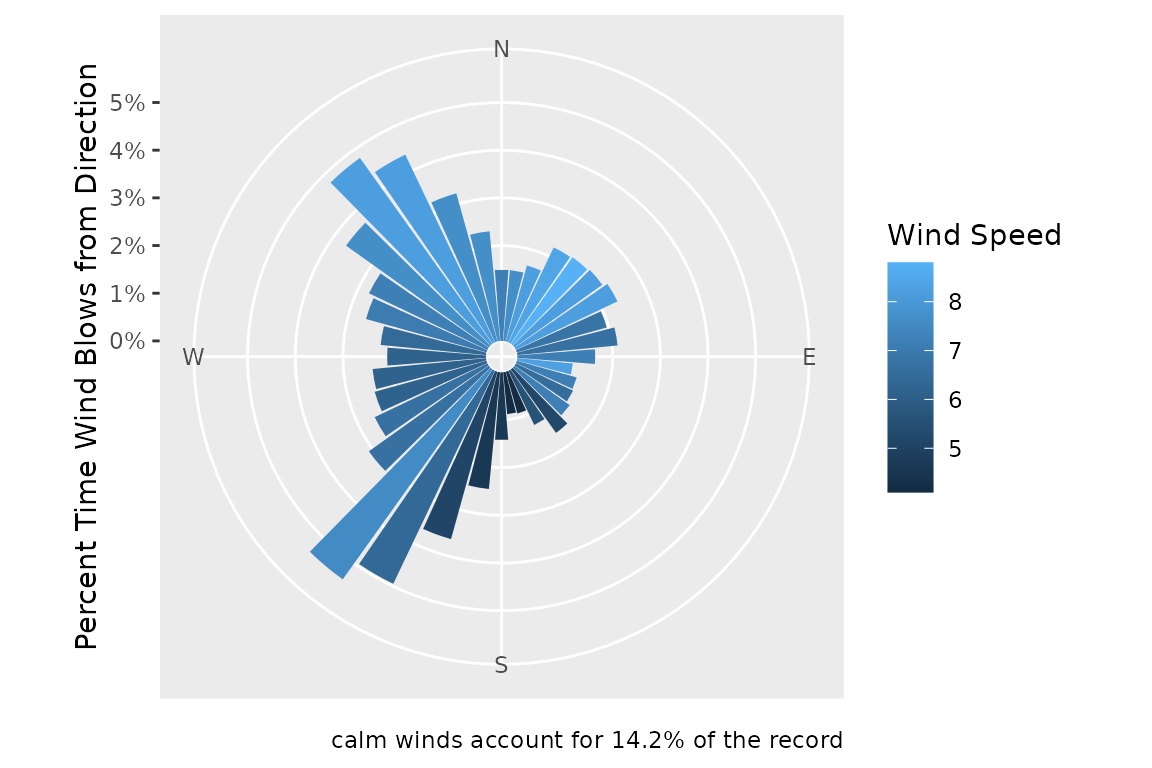

Plot showing a Wind Rose

Input wind_direction values are coerced into values 0 - 359.9. The function can further snap input wind_directions to a user supplied vector of suitable directions (directions). Input wind_directions are rounded to the nearest value in directions. This is often necessary with input data from public data sets that have occasional anomalous readings. If directions is not supplied the output is based on all unique values in wind_data$wind_direction.

The function will accept wind_percentile values from 0 to 1 or "mean". The returned speed value indicates the corresponding stat of all observations from that direction.

NA values in the wind_direction column indicate calm data if the wind_speed column is 0. However, NA values in the wind_speed column are considered bad data and are removed when wind_speed_na.rm = TRUE (the default).

Saving Wind Data

You can save wind data to as a csv file to be used with other analyses.

# Check if "data" folder exists, create if not
if (!dir.exists("data")) {
  dir.create("data")
}

# save the wind data as a .csv file
write.csv(wind_data, file = "data/wind_data.csv")

# save the summarized wind data
write.csv(wind_data_summary, file = "data/wind_data_summary_.csv")

Bathymetry

There are plenty of sources of bathymetric data and it would be impossible to discuss them all here, however NOAA’s Bathymetric Data Viewer (https://www.ncei.noaa.gov/maps/bathymetry/) offers an easy to access and interactive viewer to find some of the best publicly available datasets.

WEMo contains a convenience function get_noaa_cudem() to fetch bathymetric data from NOAA’s Continuously Updated Digital Elevation Model (CUDEM). This function accesses data from NOAA’s Continuously Updated Digital Elevation Model (CUDEM), specifically the 1/9 Arc-Second Resolution (approx. 3 meter) Topobathymetric dataset https://chs.coast.noaa.gov/htdata/raster2/elevation/NCEI_ninth_Topobathy_2014_8483/. This function takes a input point and radius and downloads topo-bathy .tif raster tiles that intersect that radius.

# extract lon and lat from our site_point
lon = sf::st_coordinates(site_point)[1]
lat = sf::st_coordinates(site_point)[2]

# download, mosaic and crop CUDEM rasters for our area of interest
bathy <- get_noaa_cudem(
  lon = lon, 
  lat = lat, 
  radius_m = 15000,
  dest_dir = "data/NOAA_CUDEM",
  mosaic_and_crop = TRUE,
  output_file = "Sinepuxent_Bathy_Cropped.tif", 
  overwrite = F
)
#> Downloading: https://noaa-nos-coastal-lidar-pds.s3.us-east-1.amazonaws.com/dem/NCEI_ninth_Topobathy_2014_8483/chesapeake_bay/ncei19_n38x25_w075x25_2019v1.tif
#> Downloading: https://noaa-nos-coastal-lidar-pds.s3.us-east-1.amazonaws.com/dem/NCEI_ninth_Topobathy_2014_8483/chesapeake_bay/ncei19_n38x25_w075x50_2019v1.tif
#> Downloading: https://noaa-nos-coastal-lidar-pds.s3.us-east-1.amazonaws.com/dem/NCEI_ninth_Topobathy_2014_8483/chesapeake_bay/ncei19_n38x50_w075x25_2019v1.tif
#> Downloading: https://noaa-nos-coastal-lidar-pds.s3.us-east-1.amazonaws.com/dem/NCEI_ninth_Topobathy_2014_8483/chesapeake_bay/ncei19_n38x50_w075x50_2019v1.tif
#> Download complete
#> |---------|---------|---------|---------|=========================================                                          
#> Cropped mosaic saved to: data/NOAA_CUDEM/Sinepuxent_Bathy_Cropped.tif

# plot the cropped raster in relation to our site point
ggplot() +
  geom_spatraster(data = bathy) +
  geom_sf(data = site_point, color = 'red', size = 5)
#> <SpatRaster> resampled to 501015 cells.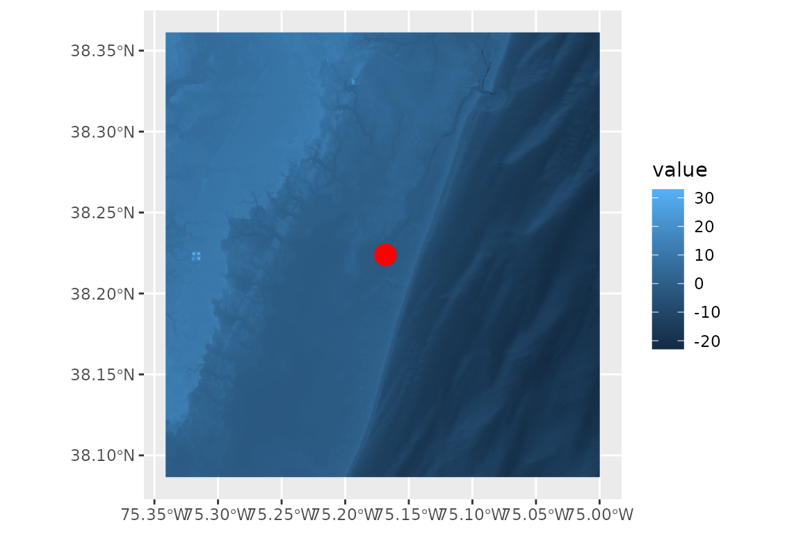

Map showing bathymetric raster around point of interest

The CUDEM dataset accessed by this function covers select areas of the United States, including:

The East Coast
The Gulf Coast
The San Francisco Bay
Part of the Oregon Coast and the Washington Coast
The Puget Sound, Washington
Portions of Cook Inlet, Alaska

Additional CUDEM products, with varying spatial resolutions and geographic extents, are available at: https://www.ncei.noaa.gov/products/coastal-elevation-models

With mosaic_and_crop = TRUE the function will stitch together the downloaded rasters and crop them to an area defined by the radius_m. This is useful for speeding up processing time by keeping the inputs to WEMo as small as possible.

With radius_m = 15000 all topo-bathy data that is within 15,000 meters of our point is fetched. This value was chosen so that the default max fetch distance that WEMo uses (10,000) will be covered by the raster after additional points in a grid of points 500 by 500 meters around this point is created further down the workflow. [need editing for clarification here?]

With overwrite = TRUE all intersecting rasters will be re-downloaded even if they are already present in the folder. Set overwrite = FALSE to skip re-downloading and increase speed.

NOTE: that dest_dir will create a folder in your working directory if one with that name doesn’t exist. You can use getwd() to determine where your working directory is. You can also include the full path to your desired folder if that isn’t in your working directory. The cropped mosaic raster is also saved to dest_dir.

Project Bathymetry

The raster generated from get_noaa_cudem() is un-projected (WGS84). WEMo requires a projected coordinate reference system with units in meters. We’ll convert the bathy to a local UTM grid (18N for our site in Sinepuxent Bay, Maryland)

# Convert to UTM Zone 18N EPSG:26918
bathy <- terra::project(
  bathy,
  "epsg:26918",
  filename = "data/Sinepuxent_Bathy_Cropped_UTM.tif",
  overwrite = T
)

Shoreline

Once you have bathymetry data, use generate_shoreline_from_bathy() to generate a shoreline based on a user defined elevation contour. We’ll use Mean Sea Level at a nearby NOAA Water Level Station: Ocean City Inlet, MD (Station ID: 8570283) to draw the shoreline for the analysis.

# MSL at Ocean City Inlet - for the shoreline definition and for use later in the workflow
water_level <- -0.141 # meters NAVD88 (match the bathy data)

# Generate Shoreline and save output to file
shoreline <- generate_shoreline_from_bathy(
  bathy = bathy,
  contour = water_level,
  save_output = TRUE,
  filename = "data/Shoreline_MSL.shp"
)
#> |---------|---------|---------|---------|=========================================                                          |---------|---------|---------|---------|=========================================                                          

# plot the shoreline
ggplot() +
  geom_sf(data = shoreline) +
  geom_sf(data = site_point, color = 'red', size = 5)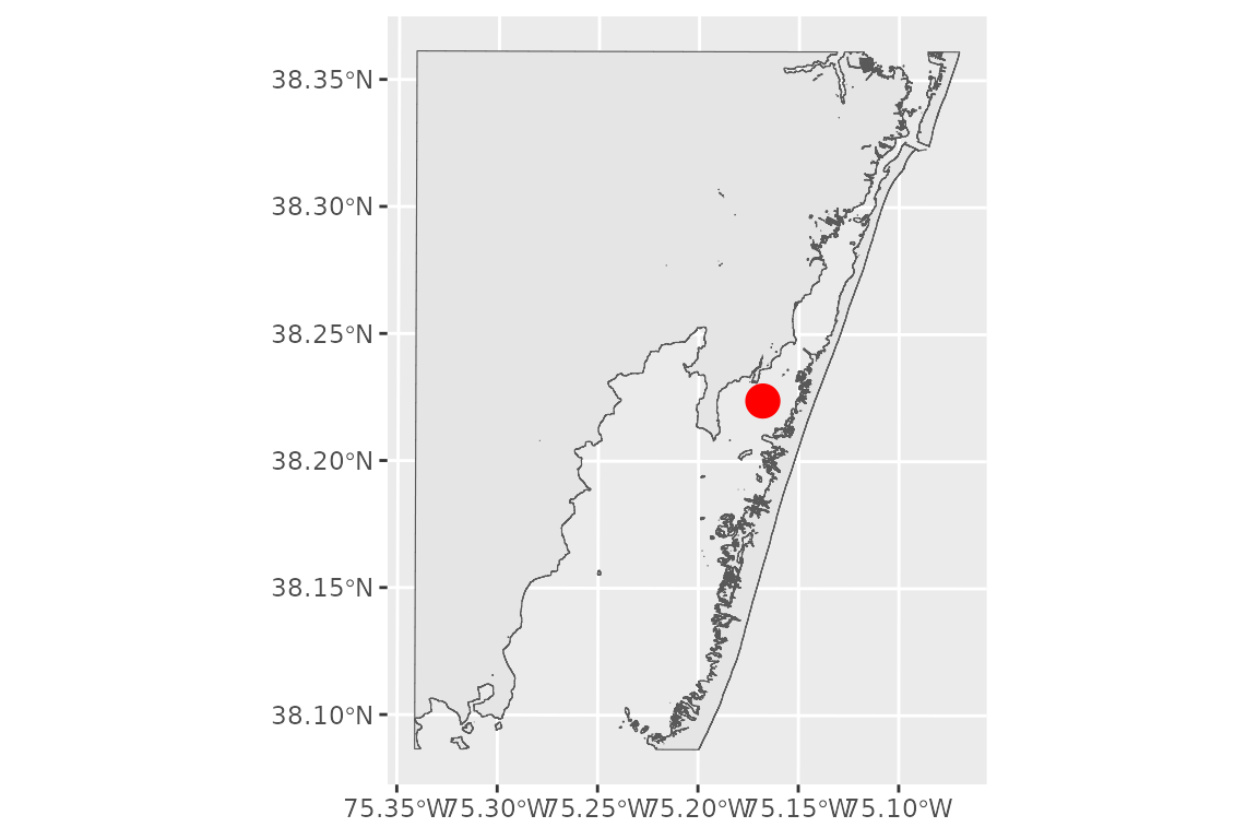

Map showing the shoreline polygon

This shoreline will define the maximum extent of the fetch rays that WEMo calculates. Selecting the proper contour to draw the polygon is critical to your analysis workflow and depends on your question. You can find a listing of stations and their published datums from NOAA CO-OPS’ National Water Level Observation Network online: https://tidesandcurrents.noaa.gov/stations.html?type=Datums. Additionally NOAA’s vdatum tool will produce datums for your area as well: https://vdatum.noaa.gov/.

Be sure to match the units and vertical datum to your bathymetry data. Bathymetry data from get_noaa_cudem() is in meters relative to NAVD88.

Grid of Points

Use generate_grid_points() to generate a rectangular grid of points. These are the points where WEMo will simulate wave exposure.

# convert the site_point to a utm grid to work with meters
site_point <- sf::st_transform(site_point, crs = 26918) # NAD83 / UTM zone 18N

# create a grid of points 500 x 500 meters with points every 100 meters
grid_points <- generate_grid_points(
  site_point = site_point,
  expansion_dist = 500,
  resolution = 100
)

# plot the grid with the original site point
ggplot() + 
  geom_sf(data = grid_points)+
  geom_sf(data = site_point, color = 'red', size = 5)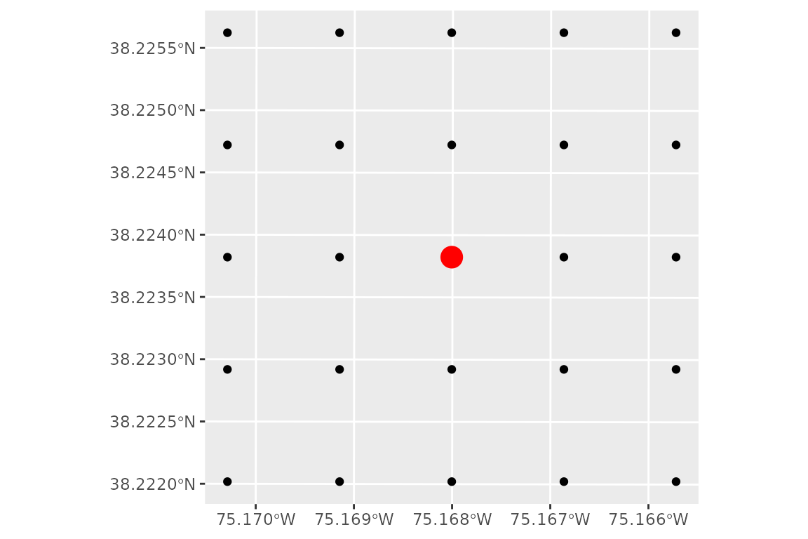

map showing the generated grid of points

If expansion_dist or resolution is a vector of length 2 the x and y expansion distances or grid resolution are set independently.

Plotting

Create a plot with all the inputs together

ggplot() +
  geom_spatraster(data = bathy) +
  geom_sf(data = shoreline, fill = "honeydew3") +
  geom_sf(data = grid_points, color = 'red') 
#> <SpatRaster> resampled to 501215 cells.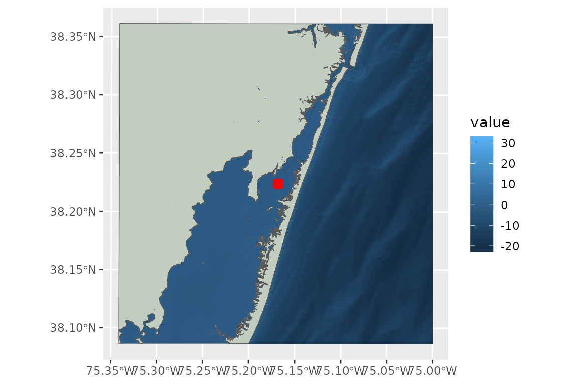

Map showing all the inputs together

All the inputs align, but it is difficult to see our points and the bathymetry color scale is stretched out by the high elevation cells on land and the low elevation cells offshore.

We can constrain the input data to fix these problems and make a nice plot:

# Get extent of the grid points
grid_ext <- terra::ext(grid_points)

# Expand the extent by 1500 meters in all directions
exp_dist = 1500

buffered_ext <- terra::ext(
  grid_ext$xmin - exp_dist,
  grid_ext$xmax + exp_dist,
  grid_ext$ymin - exp_dist,
  grid_ext$ymax + exp_dist
)

# crop the bathy to a smaller area
plot_bathy <- terra::crop(x = bathy, y = buffered_ext)

# set all cells in the bathy above our water level to NA
plot_bathy[plot_bathy > water_level] <- NA

# crop the shoreline to a smaller area
plot_shoreline <- st_crop(shoreline, buffered_ext)
#> Warning: attribute variables are assumed to be spatially constant throughout
#> all geometries

# plot
ggplot() +
  geom_spatraster(data = plot_bathy) +
  geom_sf(data = plot_shoreline, fill = "honeydew3", color = NA) +
  geom_sf(data = grid_points, color = "red") +
  coord_sf(expand = FALSE) +
  theme_bw()+
  scale_fill_viridis_c(option = 'mako', na.value = NA)+
  labs(fill = "Bathymetry (m NAVD88)")
#> <SpatRaster> resampled to 501264 cells.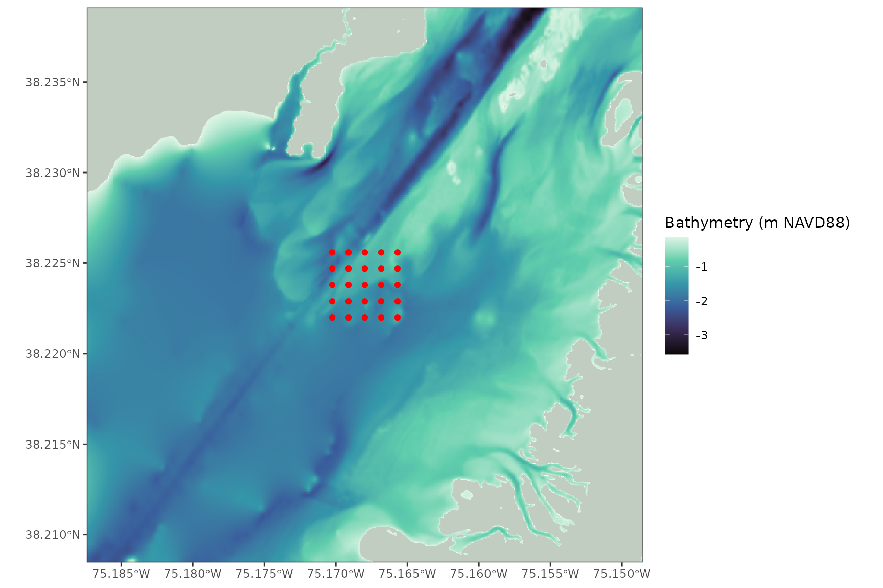

Fancy plot showing all the inputs together

That’s a pretty plot

Run WEMo model

The input data is now ready for WEMo:

# run WEMo at each of the 36 grid points that we made
results <- wemo_full(
  site_points = grid_points,
  shoreline = shoreline,
  bathy = bathy,
  wind_data = wind_data_summary,
  directions = wanted_directions,
  max_fetch = 10000,
  sample_dist = 10,
  water_level = water_level,
  depths_or_elev = 'elev'
)